What this chapter covers
This chapter explains the KPI calculation model from source production data to a stored result and its analytical representation. Before you start, make sure that the KPI microservice is installed, connected to DPA Host and synchronized as described in the DPA Installation and Operations Guide.
1. KPI: from source data to a result
KPI in DPA builds Derived values from data that changes over time. This means that a calculation is based not on a ready-made number “for the shift”, but on a time history: Indicator values, equipment states, journal records and other available sources. KPI receives this data from DPA Host, transforms it with formulas and can store the calculated time series in its own storage. When a user requests a result for a day, shift or another period, KPI aggregates the prepared history within the boundaries of that period.
Calculations are grouped in a KPI context. A KPI context defines the Work centers for which calculation is performed, the source values used, the derived values built from them and where the history is stored. A running KPI context continues calculating as new source data appears. Analytics later queries the accumulated history and can request different periods without rereading the entire source history from DPA Host.
In this chapter, we will distinguish two kinds of result. A time series is a value defined over time intervals and able to change from one interval to the next. An aggregate value is a single number calculated for a selected period. This distinction matters: a time series can serve as source history for subsequent calculations, while an aggregate value answers a question about one particular selected period.
Example: percentage of time in the Production state
Consider one Work center. Suppose the source value ProductionSignal is 1 while the equipment is in the required production state and 0 at all other times. This value is a time series: it has different values over different intervals.
In the KPI context, create a Derived value named IsProduction with the formula:
| |
The result of this formula is also a time series of zeros and ones. If storage is enabled for IsProduction, KPI records the calculated intervals in its storage. For example, during the eight hours under consideration, the value 1 might occupy 5.5 hours in total and the value 0 the remaining 2.5 hours.
To obtain one value for the selected period, create an aggregating Derived value named ProductionPercent with the formula:
| |
Here, avg calculates the average with interval duration taken into account. The average itself is a fraction from 0 to 1; multiplying by 100 converts it to the familiar numerical percentage. For the eight-hour period in the example, the result is
| |
Without multiplication by 100, the same result would be written as 0.6875. In other words, ProductionPercent answers the question “for what share of the selected time was IsProduction equal to one?” If the user selects a different period, KPI calculates a different aggregate from the same stored history. ProductionPercent itself does not form a continuous time history: the aggregating formula is evaluated for the requested period.
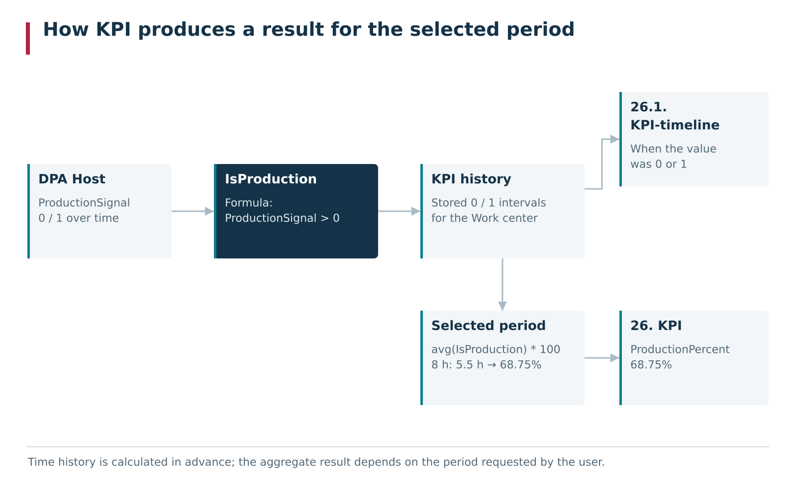
KPI path from source time history to the result for a selected period. The IsProduction time series is calculated and stored as data arrives, while ProductionPercent is evaluated by an aggregating formula for the period selected by the user.
The same calculation therefore contains two different kinds of result. IsProduction describes what happened over time and can be stored as a sequence of intervals. ProductionPercent answers what the aggregate is for a particular period and is calculated when analytics is requested. This distinction becomes important when configuring formulas and choosing a view.
Analytics → 26.1. KPI-timeline is intended for viewing time series and helps show when a calculated value changed. Analytics → 26. KPI reduces the selected period to aggregate values. The same KPI context can therefore prepare interval history for later analysis while also defining values that become meaningful only after a period is selected.
The following sections explain the contents of a KPI context, sources of time-based data, types of calculated values and the formula language. For now, keep the overall chain in mind: source data → time series → calculated time series → stored history → aggregation of the selected period → analytical representation.
2. Readiness
KPI is a separate DPA microservice. Before calculations can be configured, it must be installed, connected to DPA Host and reachable over the network. Installation, microservice registration and connection setup are described in the DPA Installation and Operations Guide. In this chapter, we assume that the technical connection has already been completed.
Access to configuration and viewing
To change KPI settings, the user needs access to the general DPA settings and the Manage OEE settings permission. The View OEE permission is used to view the configuration and results.
Source data must exist over time
KPI calculation starts with time history. For the selected Work centers, the source data used by the KPI context must exist: for example, Indicator values, equipment states or records from other supported DPA Host sources. If a Basic value is linked to an Indicator, that Indicator must be correctly assigned for every Work center included in the calculation.
It is important to distinguish the value 0 from missing data. Zero is an ordinary time-series value
and participates in calculations. A missing interval means that KPI has no source value over that
part of the timeline. Time-series formulas do not automatically substitute zero for such an interval,
so incomplete source history can produce incomplete calculated history and results that cannot be
interpreted as calculations over the entire requested period.
Also consider the time boundaries of the KPI context itself. History does not appear before the point from which the KPI context began receiving and calculating it, while data too close to the current time may not yet be requested because of the configured delay. These settings are described in detail in section 3, “KPI contexts”.
Control check of a calculation
For the first check, it is convenient to use a Work center and a source value whose history can be viewed independently in DPA Host. Create or select a simple KPI context, start it and wait until a known part of the history has been processed. Then check not only the state of the KPI context, but the calculation result itself:
- in
Analytics → 26.1. KPI-timeline, make sure that intervals for a simple calculated time series have appeared over the expected part of the timeline; or - in
Analytics → 26. KPI, request a period for which the expected aggregate is known in advance and compare the value with the source history.
A KPI context state of “running” means that the KPI context is not stopped, but it does not guarantee that every source is available, every formula has been built successfully or all time series are advancing. The control check should therefore reach an actual interval or aggregate value. Once that check succeeds, you can proceed to configuring the working KPI context.
3. KPI contexts
A KPI context combines one calculation model: a set of Work centers, input Basic values, Derived values built from them, additional Data slices and storage for the calculated history. KPI contexts are independent of one another, so one installation can maintain several KPI sets with different sources, formulas, equipment and time boundaries.
Open KPI from the Applications menu. On the Context list tab, each KPI context shows its Start date, State, Storage, and the number of included Work centers, Basic values, Data slices and Derived values. Commands above the table let you create, edit, restart, clone or delete the selected KPI context.

List of KPI contexts. For each KPI context, the start date, state, storage and number of Work centers, Basic values, Data slices and Derived values are shown.
The indicator in the State column shows whether the KPI context is enabled. Restart context rebuilds the running calculation, but it does not by itself delete stored history and it is not a full recalculation command. These differences are explained in detail in section 7, “Calculation and recalculation”.
Cloning creates a new KPI context with the same configuration and a new name. The copy is created stopped; the stored history of the source KPI context is not copied. Deleting a KPI context, on the other hand, deletes its associated value configuration and stored values, so use this command only after checking the selected row.
Context contents
Open a KPI context by double-clicking its row or by using Edit. General settings are at the top of the form, followed by five tabs containing the context configuration.
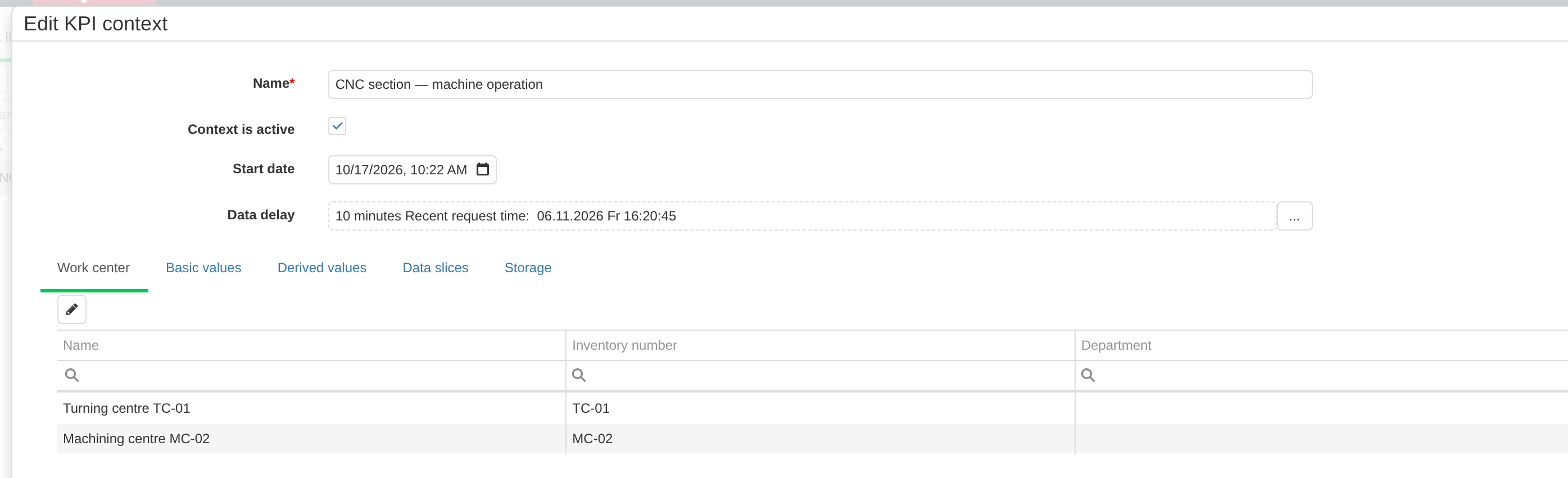
The KPI context form combines general calculation settings and five tabs: Work center, Basic values, Derived values, Data slices and Storage.
The tabs have the following roles:
- Work center — the equipment for which the calculation is performed. KPI maintains separate instances of the context’s time series for every selected Work center;
- Basic values — input time series that KPI receives from DPA Host;
- Derived values — values built by formulas from Basic values and other Derived values;
- Data slices — additional time-dependent attributes that can divide results into groups in analytics;
- Storage — where the KPI context history is stored and where operations on that history are queued.
Basic values are described in detail in section 4, “Basic values and source time history”, and Derived values in section 5, “Formulas”. At this point, the important thing is the boundary of a KPI context: the selected Work centers, all its values and the stored history form one consistent calculation set.
Context name and activation
The Name field is used to select the KPI context in settings and analytics. Give KPI contexts names that make the purpose of the calculation clear, for example “Equipment states”, “Shop OEE” or “Energy consumption”.
The Context is active checkbox controls whether calculations run. An active KPI context starts and continues receiving new source data; an inactive KPI context does not advance its calculations. Stopping a context does not delete history that has already been stored, so previously calculated intervals remain in storage until a separate deletion operation is performed.
When some settings of an active KPI context are saved, the UI offers to restart the context so that the new configuration takes effect in the running calculation. If you decline that restart, the saved configuration and the already running calculation may temporarily differ. Therefore, after changing sources, formulas, storage or other settings for which this prompt appears, restart the KPI context before performing a control check of the result.
Start date
Start date sets the lower time boundary before which the KPI context should not begin retrieving and building its history. For a new KPI context, this is the starting point of the calculation, not the period displayed in analytics. The period in Analytics → 26. KPI and Analytics → 26.1. KPI-timeline is selected separately.
If a KPI context already has stored history, changing Start date does not by itself clear or recalculate that history. KPI continues to take into account the stored boundary of each individual time series. Treat changing the start date and recalculating history as separate operations; safe recalculation options are described in section 7, “Calculation and recalculation”.
Data delay
Data delay determines how close to the current time KPI requests source data from DPA Host. The default delay is 10 minutes. For example, with this setting, at 14:30 KPI requests history only up to approximately 14:20, leaving the most recent minutes for the source to form and store its data. The field next to the delay shows the time of the nearest available request.
Data delay is not the polling frequency. It defines a time boundary — “not closer than this to the current moment” — while the Polling interval of a particular Basic value determines how often KPI repeats requests to its source. These settings solve different problems.
The Data delay dialog can supplement the ordinary absolute delay with a calendar rule. The Is active checkbox enables this rule. A number and the adjacent list define a calendar boundary in days, weeks or months, and the time field specifies the point within the selected calendar period. For example, the combination 0 days ago (today) and 00:00 limits requests to the start of the current day. KPI compares the calendar boundary with the absolute delay and uses the more conservative one.
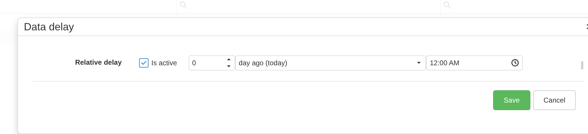
The Relative delay calendar rule: Is active enables the rule, the number and list define the calendar period, and the time field sets the boundary within the selected period.
Work centers as the calculation scope
On the Work center tab, select the equipment to which the KPI context applies. One KPI context can include several Work centers. KPI calculates a separate time history of every value for every selected Work center. Normally they use one primary formula; when necessary, a Derived value can have an additional formula for particular Work centers. This setting is shown in section 5, “Formulas”. This is why analytics can show both each Work center result and a total result for a selected equipment group.
For Basic values based on Indicators, the particular Indicator can differ between Work centers. The mapping is configured in the Basic value; the KPI context only defines the equipment set for which that mapping must be complete.
A KPI context therefore does not define one ready-made KPI. It defines the boundaries of an entire calculation model: equipment, time start and delay, input and calculated time series, grouping rules and the history storage location. The following sections examine the contents of that model separately.
4. Basic values and source time history
A Basic value is a named input time series in a KPI context. Derived values refer to it by variable name and receive values that KPI requests from DPA Host for each Work center. Configuring a Basic value therefore answers two questions at once: what data to retrieve and how often to check for new history.
Open the KPI context, go to the Basic values tab and click the add button. Variable name defines the name later used in formulas. The name must start with a letter and may contain letters, digits and underscores; spaces are not used. Within one KPI context, Basic value and Derived value names must be unique. For example, you can use ShiftTime for shift working time and Feed for feed rate.
Basic value type offers two ways to obtain a source time series:
- Basic Value — a ready-made DPA Host source that already represents production data in a form suitable for KPI;
- Indicator — direct reading of a selected Indicator for each Work center.
Both methods create a time series. Only the source of its values differs.
Ready-made DPA Host sources
For the Basic Value type, select the source in the Basic Value field. The list includes, for example, actual and planned operation time, produced quantity, shift working time, Work center states and modes, different kinds of downtime and other production data. Use a source whose meaning matches the value you want to calculate instead of rebuilding the same business logic from lower-level data.
Some sources have additional parameters. They appear in the form after a source is selected. For example, Shift working time requires a particular shift to be selected. The set of fields therefore depends on the selected source.
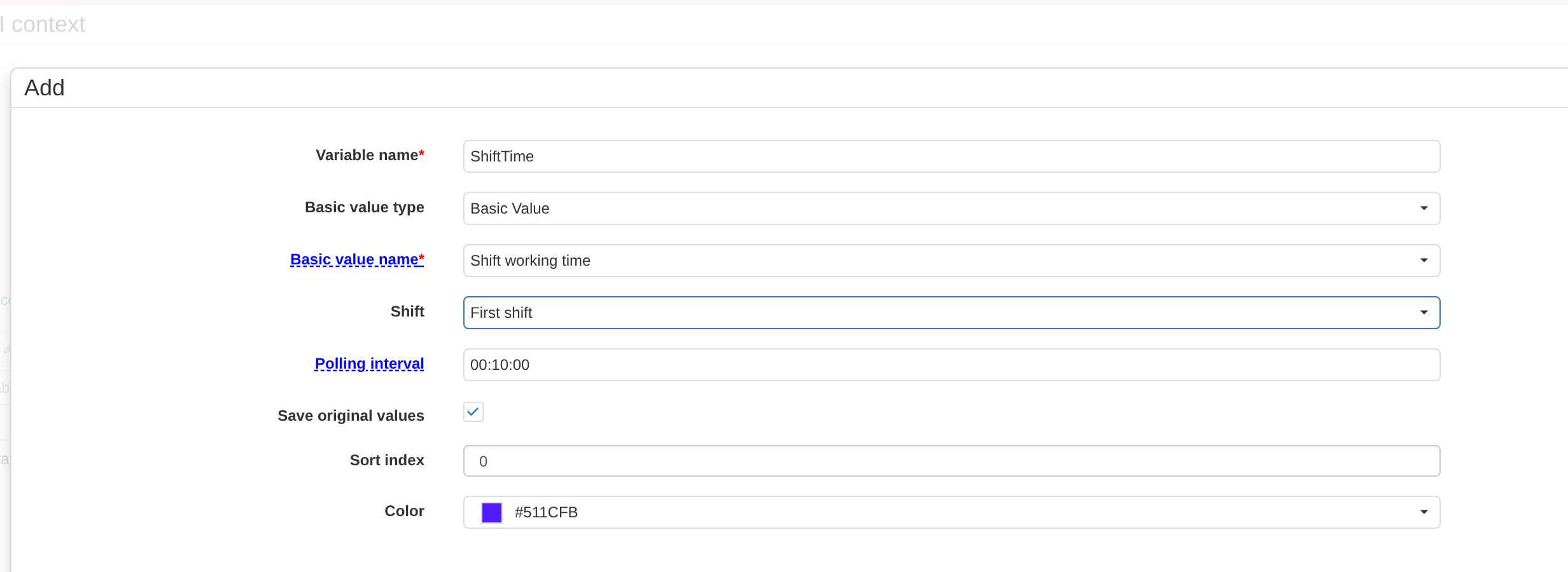
A Basic value from a ready-made DPA Host source. After Shift working time is selected, the form shows the additional Shift parameter; the other settings control polling interval, storage and presentation of the value.
A ready-made source defines not only where data is obtained but also the meaning of the returned time series. One source may return a binary 0/1 value, another a quantity, duration, mode or numerical production value. Before using such a series in a formula, make sure that you understand its unit of measurement, when applicable, and what its value represents.
Work center Indicators
Select the Indicator type when the source value should come from an existing equipment Indicator. The form then shows a table of all Work centers in the KPI context. Select an Indicator for each Work center.
This mapping is configured separately for every Work center: a single variable such as Feed can read different Indicator instances on different machines. Formulas in the KPI context can therefore use the common name Feed, while KPI substitutes the appropriate source for the particular equipment. Before saving, complete the mapping for every Work center in the KPI context.
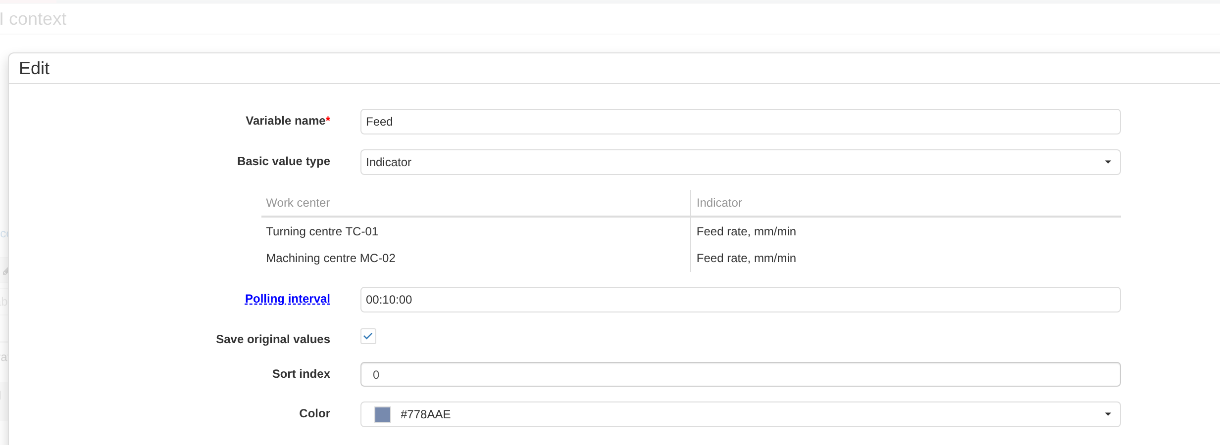
A Basic value of the Indicator type. The same variable name Feed is mapped to an Indicator separately for every Work center in the KPI context.
If the equipment set of a KPI context changes, check the Indicator mappings of its Basic values: every new Work center must also receive a source for each variable of the Indicator type.
Polling interval and storing source values
Polling interval defines how frequently this Basic value requests data from DPA Host. The value must be at least 10 seconds; the UI recommends an interval between 1 and 10 minutes. A short interval picks up new data sooner but produces more requests. A long interval reduces request frequency and increases the delay before new values appear in KPI. KPI continues requesting history from the already processed time boundary, so less frequent polling does not by itself mean that intermediate data is skipped.
Do not confuse Polling interval with the KPI context Data delay. The delay determines how close to the current moment history may be requested, while Polling interval determines how often a particular Basic value repeats its request.
The Save original values checkbox determines whether the retrieved time series is stored in KPI storage. A stored Basic value can later be used as an independent historical time series in analytics and aggregation. If storage is disabled, the value can still participate in the current calculation of dependent time series, but its own numerical intervals are not retained as historical data. Disable storage only when the source series is an intermediate input and the history needed for later analysis is stored in Derived values.
Sort index and Color affect how the value is presented and do not change its numerical values.
Zero and a missing time interval
KPI makes an essential distinction between the value 0 and a missing value. Zero is an ordinary time-series number. If a source returns an interval with value 0, that interval exists and participates in subsequent formulas and aggregations.
A missing interval means that KPI has no value for that series over that portion of time. KPI does not automatically substitute zero for a missing interval. If a formula uses several time series, the result is built only where the required input values exist. A gap in one Basic value can therefore create a gap in dependent Derived values as well.
For example, if Feed has continuous history for eight hours but a second formula input is missing for a twenty-minute interval, the combined calculation does not automatically treat those twenty minutes as zero. In analytics, the result then represents only the portion of history that was actually calculated. Checking coverage duration with dur is discussed in section 5, “Formulas” and section 6, “Practical calculation techniques”.
The quality of source time history should therefore be checked before formulas are made more complex. For every Basic value, its source, unit of measurement (if applicable), value semantics, equipment mapping and expected time coverage should be clear. Subsequent Derived values then work with well-defined input series, and a missing result can be traced through the dependency chain.
5. Formulas
A Derived value defines a named value that KPI builds by formula from Basic values, other Derived values and numeric constants. Open a KPI context, go to the Derived values tab and add a new value. In Variable name, enter the name by which subsequent formulas can refer to it; in Function, enter the calculation expression.
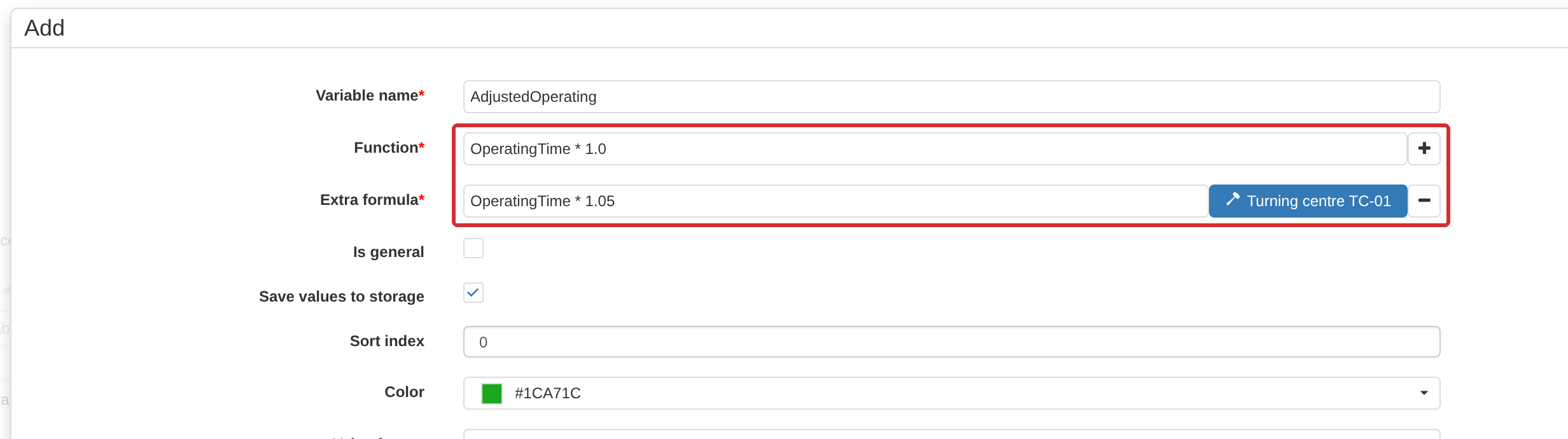
The Derived value form. Function defines the main formula, while the + button adds an Extra formula for selected Work centers. Is general and Save values to storage control whether the result is used in summary analytics and whether the calculated time series is stored.
The variable name must start with a letter and may contain letters, digits and underscores. Basic value and Derived value names share the same namespace within a KPI context, so they must not duplicate one another. The formula editor suggests available variables and functions while you type.
The Is general checkbox includes a Derived value in the result set used by the summary analytics Analytics → 26. KPI. If a general value remains a time series, KPI automatically calculates its average over the selected period when an aggregate value is requested. If the aggregate should have another meaning — for example a sum, duration or ratio of several aggregates — define that explicitly with an aggregating formula.
The Save values to storage checkbox is meaningful for a formula that creates a time series: the calculated intervals of that value are stored and can be used by later calculations and analytics. If an intermediate time series must later participate in avg, sum or dur over an arbitrary period, store it: aggregation is performed over stored history. A formula that already reduces a series to one aggregate for a period does not create separate interval history; enabling storage does not turn such an aggregate into a time series.
Sort index, Color, Value format, Display name, Values group and Equipment values group control how the result is presented in analytics and do not change the mathematical meaning of the formula. These fields are used in section 8, “Analytics ‘26. KPI’” and section 9, “Analytics ‘26.1. KPI-timeline’”.
Time series and aggregate for a period
KPI formulas fall into two fundamentally different kinds.
A time-series formula is evaluated over time. For example, Feed * 0.1, Temperature - 20 or ProductionSignal > 0 create a new series of intervals. Such a Derived value can be used by other time-series formulas and, when storage is enabled, has its own history.
An aggregating formula, directly or through a dependent value, uses avg, sum or dur and reduces a time series to one number for the period requested by analytics. For example, the formula introduced at the beginning of the chapter,
| |
returns the share of time during which IsProduction = 1 within the selected period, expressed as a percentage. The value depends on the request boundaries: a shift, day and week may produce different results.
As long as an expression remains time-based, time series can be combined with one another in the ordinary way: added, subtracted, multiplied, divided, compared and passed to numeric functions. For example, A + B, A * B and max(A, B) create new time series. KPI aligns argument intervals by time and recalculates the result at each boundary where at least one input changes. A result exists only where all required arguments have coverage: a missing series is not substituted with zero.
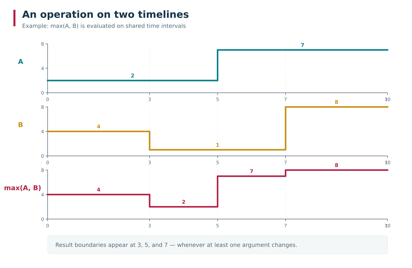
Two time series can be added, multiplied, compared and passed to ordinary numeric functions. In the max(A, B) example, KPI splits the shared time domain at boundaries from both arguments: the result changes at 3, 5 and 7 and remains a time series.
Once the calculation moves to an aggregate for a period, it operates in a different domain. An aggregated value can be combined with numeric constants and other aggregated values, but it cannot be multiplied by or added to a time series as though the aggregate automatically extended to every moment in time.
| Formula | Result kind | Comment |
|---|---|---|
A + B | Time series | The sum is calculated over every shared interval of the A and B histories. |
max(A, B) | Time series | The greater current value is selected over each shared interval. |
Feed > 0 | Time series | The comparison produces 1 or 0. |
avg(IsProduction) * 100 | Aggregate for a period | The time-weighted average is converted to a percentage. |
sum(A) / dur(A) | Aggregate for a period | Arithmetic between several aggregated values is allowed. |
avg(A) * B | Error | An aggregate for a period cannot be mixed with the time series B. |
If you need to aggregate a complex expression over time series, first create an intermediate Derived value, then aggregate that value. For example, instead of the invalid sum(A + B), create AB = A + B, store its history and use sum(AB).
Operators and ordinary numeric functions
Formulas support parentheses, unary + and -, and the following binary operators:
| Group | Operators | Result |
|---|---|---|
| Power | ^ | Exponentiation. |
| Arithmetic | *, /, +, - | Ordinary numeric operations. Division by 0 returns 0. |
| Comparison | >, >=, <, <=, ==, != | 1 if the condition is true, otherwise 0. |
| Logic | &, OR | 1 if the corresponding logical condition is true; a positive value is treated as true. |
| Substitution | ?? | A ?? B returns B only when A is missing (NaN); otherwise it returns A. |
| Filter | ? | Condition ? Value returns Value if Condition > 0; otherwise the result is missing (NaN). |
Logical OR is written with the vertical bar |.
Operator precedence runs from ^ through *//, +/-, comparisons, &, |, then ?? and ?. When order matters to the meaning of a value, use parentheses explicitly.
Ordinary numeric functions work in both the time-series and aggregated parts of an expression, provided their arguments belong to the same result kind. For time series, the function is applied to the current values over each shared time interval rather than once to the entire history: for example, max(A, B) repeatedly calculates the maximum of the current A and B values between adjacent interval boundaries.
min(a, b, ...)andmax(a, b, ...)— minimum and maximum of two or more arguments;abs(x)— absolute value;floor(x)andceil(x)— round down and up;round(x)— round to the nearest integer; halves are rounded away from zero.
Except for ?? and ?, the special NaN value inside an existing interval propagates through the expression result. Therefore, A ?? 0 can replace specifically NaN with zero. This operation does not create a time interval where A has no coverage at all: a gap in the source history remains a gap, as described in section 4, “Basic values and source time history”.
Time-series functions
The following history-processing functions remain time series:
| Function | Purpose |
|---|---|
avgWin(x, width[, step]) | Average over a time window. The average is weighted by interval duration. |
minWin(x, width[, step]) | Minimum over a time window. |
maxWin(x, width[, step]) | Maximum over a time window. |
diff(x[, overflow[, idleMinutesTimeout]]) | Rate of change; the result is normalized per hour. overflow accounts for counter rollover, while the last argument can produce 0 after the specified time with no change. |
gate(x, minDurationMinutes[, maxDurationMinutes]) | Duration filter for nonzero intervals: intervals that are too short, and when a maximum is specified those that are too long, are replaced with zero. |
Time parameters can use the suffixes sec, min and hr, for example avgWin(Feed, 10min) or avgWin(Feed, 1hr, 5min). A number without a suffix in these function parameters is interpreted as minutes. If step is omitted, it equals the window width. For avgWin, minWin and maxWin, KPI limits both window width and step to the range from 1 second to 24 hours. Parameters after the first function argument must be constants, not other time-dependent variables.
When the step equals the window width, adjacent windows do not overlap: each window becomes one enlarged output interval. When the step is smaller than the width, windows overlap and a new aggregated value appears more frequently.
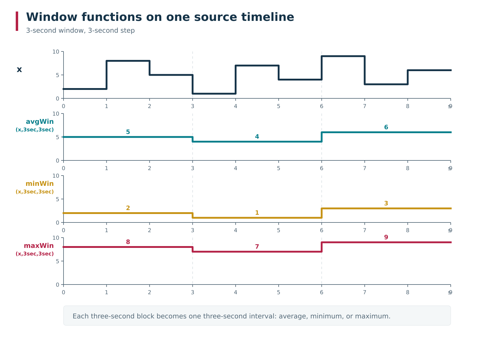
The same series is processed with a 3-second window and the same step. For every window, avgWin returns the time-weighted average, minWin the minimum and maxWin the maximum; nine one-second intervals therefore become three coarser intervals.
Smoothing and downsampling with window functions
Window width determines how much source history contributes to one result, while step determines how often the next result appears. The same avgWin can therefore solve two related but distinct practical tasks. A large window with a small step primarily smooths rapid fluctuations while retaining a frequent output time grid. A large step comparable to the window width both coarsens the history and reduces the number of stored intervals — in other words, it downsamples the data.
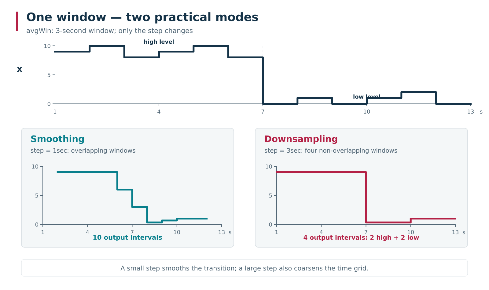
For avgWin, window width and step solve different tasks. The source series contains 12 one-second intervals: values first fluctuate around a high level and then around a low one. With a 3-second window and a 1-second step, overlapping windows smooth the transition; with a 3-second step, the same data becomes four coarser intervals — two high and two low.
For example, if one source value changes approximately once every 10 minutes and another once per second, long-term analytics does not always need the one-second series stored at its original detail. You can create an intermediate Derived value such as Fast3m = avgWin(Fast, 3min, 3min) and store that instead. With full coverage, this converts many short source intervals into one averaged interval for every three minutes. If the original fast series is not needed in stored form by other calculations, its own storage can be disabled.
Such downsampling can reduce the history volume by tens of times, but the acceptable loss of time detail depends on the signal and subsequent formulas. Check it on a representative portion of data: for some aggregates the difference will be negligible, while a nonlinear formula, threshold or short event may be sensitive to coarsening.
Aggregating functions
Three functions convert a time series into an aggregate value for the requested period:
| Function | Meaning |
|---|---|
avg(x) | Average weighted by the duration of existing x intervals. |
sum(x) | Integral of value over time: Σ(value × duration in hours). This is not a sum of discrete samples. |
dur(x) | Total duration of existing x coverage in hours. |
Each of these functions accepts one variable, not an arbitrary expression. Therefore, sum(A + 1) is invalid: first create and, when necessary, store the time series B = A + 1, then use sum(B). An already aggregated value cannot be aggregated again either.
Geometrically, the difference between avg, sum and dur is straightforward. Suppose x = 10 for the first four hours and x = 0 for the next four hours, with full eight-hour coverage. Then avg(x) = 5 is the average level, sum(x) = 40 is the area under the graph in “value × hours” units, and dur(x) = 8 is the length of the covered time interval. For a binary 0/1 series, sum(x) is therefore numerically equal to the number of hours spent in state 1.
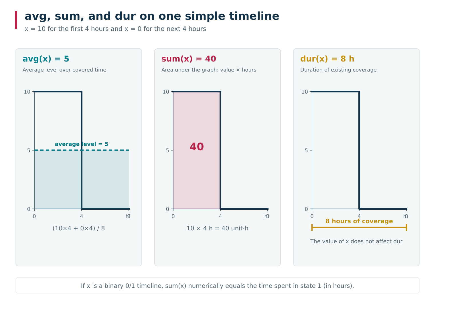
The same eight-hour series illustrates three different aggregation meanings. avg(x) gives the average level 5, sum(x) gives the area under the graph, 40 value·h, and dur(x) gives 8 hours of existing coverage regardless of the series values.
If a twenty-minute interval is missing within those eight hours, KPI does not treat it as zero. dur(x) becomes less than eight hours, while avg and sum are calculated only over the existing coverage. dur is therefore useful not only as part of a formula but also as a check of time-history completeness before an aggregate KPI is interpreted.
Additional formulas for particular Work centers
Normally Function defines one Derived value formula for all Work centers in a KPI context. In the form shown above, the + button on the right adds an Extra formula row. One or more Work centers can be selected for it: on the selected equipment the extra expression replaces the main formula, while Function continues to apply to all other equipment.
This mechanism keeps one value name and presentation when the same production meaning requires different normalization or a different expression on part of the equipment. For example, the main formula can be Working * 1.0, while one particular machine uses Working * 1.05.
A single Work center must not belong to more than one extra formula for the same value. In the extra-formula selector, choose only the equipment set that actually requires a different expression.
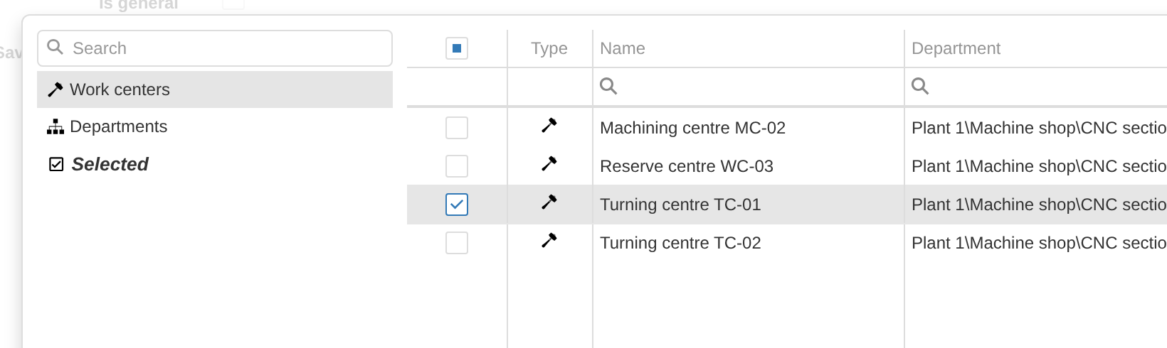
Selecting Work centers for an extra formula. The extra expression applies to the selected equipment; the main Function remains in effect for all other Work centers of this Derived value.
This capability has an important limitation: a Derived value with formulas defined for particular Work centers cannot be used as an aggregate value in Analytics → 26. KPI. Requesting an aggregate for such a value returns a formula error. Use extra formulas for calculated time series per equipment; if you need one overall aggregate KPI, bring the source series to a common formula before moving to avg, sum or dur.
Checking a formula
A formula can refer to existing Basic values and Derived values in the same KPI context. Cyclic dependencies are not allowed: for example, A = B + 1 together with B = A + 1 does not form a calculable model.
Successfully saving the settings does not guarantee that a formula is semantically valid. In particular, a configuration may be saved with an unknown variable or an invalid mix of a time series and an aggregated value, with the error appearing only when the calculation is built or when an aggregate value is requested. After changing formulas, therefore, perform a control check against a known portion of history.
If the KPI context is already active, changing a formula is one of the settings for which the UI offers a restart. Restart the KPI context so that the new formula takes effect in the running calculation. Restarting does not rewrite previously stored history using the new formula: the distinction between applying a new configuration and historically recalculating data is covered in section 7, “Calculation and recalculation”.
6. Practical calculation techniques
The KPI formula language does not need a separate built-in function for every production question. Many tasks reduce to the same few techniques: represent a condition as a 0/1 time series, use it as a mask, then aggregate the resulting history with sum, avg or dur.
The main idea of this section is that a binary 0/1 value is not only a logical state but also a convenient time mask. The value 1 marks intervals that should be included, while 0 marks intervals that should be excluded from a duration, share or weighted average.
How long a condition was true
Suppose IsProduction is 1 while a Work center is in the Production state and 0 at all other times. Because sum integrates value over time in hours, the formula
| |
returns the duration of Production in hours. For example, a result of 3.75 means 3 h 45 min. If the result is needed in minutes, multiply the aggregate by 60:
| |
The same technique works for any binary mask: setup time, downtime, time running a selected program, time within a shift and other conditions that can be represented as a 0/1 time series.
What share of time a condition was true
For a binary series M, the time-weighted average directly equals the share of covered time for which M = 1:
| |
With full coverage of an eight-hour period in which M = 1 for five hours, the result is 0.625, or 62.5%. An equivalent expression shows the relationship among the three aggregators:
| |
Here, sum(M) is the number of hours in state 1, while dur(M) is the entire history of M that actually exists. With data gaps, avg(M) and sum(M) / dur(M) therefore still describe the share of covered time, not automatically the entire requested period.
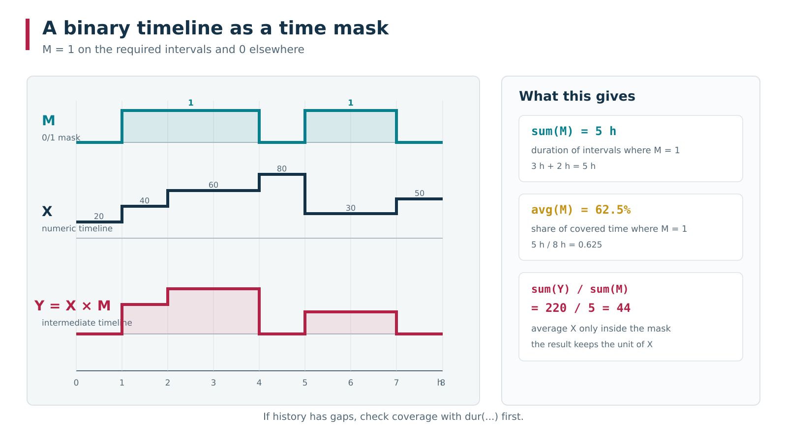
A binary time series M works as a mask: sum(M) gives the hours spent in state 1, while avg(M) gives its share of covered time. If you create the time-based value Y = X * M, it keeps X only on the selected intervals; sum(Y) / sum(M) then gives the average of X within the condition.
Share of a state within shift time
To answer “what share of the shift was the machine in Production?”, use two masks:
IsShift = 1within the required shift and0outside it;IsProduction = 1in Production and0in all other states.
First restrict Production to shift time:
| |
ProductionInShift is a time-based Derived value. Store it if the aggregate must be calculated for arbitrary periods. Then define the aggregate as
| |
The numerator is the number of Production hours within the shift; the denominator is the number of hours in the shift itself. Multiplication by 100 converts the fraction to a percentage. Explicit multiplication by IsShift is safer than simply using sum(IsProduction) / sum(IsShift): it filters out Production intervals outside the selected shift if such intervals can exist in the source history.
The same pattern produces “downtime share of shift”, “setup share of available time” and other ratios of two durations. First build masks for the numerator and denominator, then divide their sum values.
Average of a numeric value only within a required state
Suppose Feed is feed rate and you need its average only during Production. First create the time-based value
| |
then the aggregate:
| |
This is an ordinary time-weighted average. In the numerator, one unit of Feed is multiplied by hours; the denominator contains hours, so the result returns to the original Feed unit.
This recipe assumes that Feed has valid coverage wherever IsProduction = 1. If the numeric series contains gaps, check its coverage first: otherwise the denominator may include time for which no numeric value actually existed.
Checking time-history completeness
dur(X) returns the duration of existing X coverage in hours, regardless of the values in the series. This is a simple diagnostic technique before interpreting aggregates.
For example, if 12 hours of history are expected for the selected period but
| |
returns 9.5, Feed has only 9 h 30 min of coverage. Zeros inside the series do not affect dur: an interval whose value is 0 exists and counts toward duration, while a real history gap does not.
When several inputs are compared, it is useful to check dur for each. If a formula depends on A and B and their coverage differs, the resulting time series exists only over the shared portion of their histories.
Ratio of two durations as a general pattern
Many production KPIs have the same structure:
| |
where both variables are 0/1 time masks. If the numerator domain must also be restricted to the denominator domain, first build their intersection:
| |
then use sum(NumeratorInScope) / sum(DenominatorMask). This single pattern covers many utilization, availability and time-share values without requiring a special function for every business question.
7. Calculation and recalculation
An active KPI context has two related but distinct states: the running calculation and stored history. The running calculation receives new Basic values, builds dependent time series and advances forward. Stored history lets calculation resume from an already reached time boundary after a stop and later provides aggregates for arbitrary periods.
This leads to an important practical distinction: restarting a KPI context is not the same as historical recalculation. A restart rebuilds the running calculation model from the current configuration, but it does not delete intervals that have already been stored. Historical recalculation begins only after the required portion of stored history has been deleted so that KPI can build it again.
How calculation continues
For every Work center, KPI maintains separate instances of stored time series. When a KPI context starts or restarts, it first uses the existing history of each stored series and then continues from the time boundary already reached. Stopping a KPI context therefore does not by itself mean data loss or rereading the entire history from Start date.
Basic values continue requesting new source intervals according to Data delay and their own Polling interval. Time-based Derived values are built wherever the necessary input coverage exists. If storage is enabled, calculated intervals become the new stored boundary of that value.
Aggregating formulas avg, sum and dur work differently: they do not create a separate stream of intervals, but calculate an aggregate for the period requested by analytics. Such calculations use stored time series as described in section 5, “Formulas”.
An ordinary restart is not a search-and-repair operation for arbitrary gaps inside an already stored range. If a gap appeared in the middle of history and later parts of the series are stored again, a restart alone does not have to return to that gap. To restore history, explicitly move the time boundary of the affected series backward.
Restarting a KPI context
Restart context in the KPI context list and Pause and restart on the Storage tab solve the same primary task: stop the current calculation model and rebuild it from the saved configuration.
This is required, for example, after changing a formula, Basic value source, storage mode, storage location or Data delay when the UI offers to apply the change through a restart. After restarting, new portions of history are calculated using the new configuration.
Existing stored history remains in place. If the formula Echo = Run + 1 was changed to Echo = Run + 100, an ordinary restart does not convert old stored Echo values to the new formula. The old history remains up to its existing stored boundary, and new calculation continues using the current formula. If the entire history must match the new formula, recalculation is required.
Operations on stored history
Open the KPI context, select the Storage tab and click the add button in the Data storage queued operations table. The Add operation in queue dialog provides four operations.
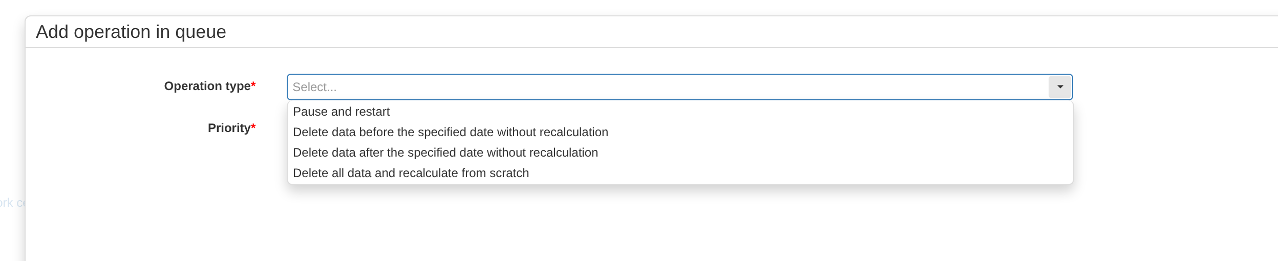
In the storage queue, restart is separated from operations on history: you can delete an older or newer portion of selected series, or clear all data and rebuild it from scratch.
| Operation | What happens to history | When to use it |
|---|---|---|
| Pause and restart | Nothing is deleted. The calculation model is rebuilt and continues from the stored boundaries. | Apply the new configuration to future calculation. |
| Delete data before the specified date without recalculation | For selected values and Work centers, the older portion of history before the boundary is deleted. The current later boundary is not moved backward. | Intentionally discard an old portion of history. |
| Delete data after the specified date without recalculation | For selected values and Work centers, history from the specified date onward is deleted. After calculation resumes, this portion can be retrieved or calculated again. | Recalculate history from a particular point in time. |
| Delete all data and recalculate from scratch | The KPI context stored history is cleared completely; an active KPI context rebuilds it from its Start date. | Bring all history in line with the current formulas and settings. |
Operations are executed through the storage queue. During an operation that modifies the current KPI context history, its calculation is paused; once the operation completes, an active KPI context resumes. Priority refers to the operation queue; for an ordinary single operation, leave it at Normal.
Deletion does not create data by itself. Only a portion for which source data is still available in DPA Host or is already stored in the KPI series being used can be rebuilt.
Recalculation from a specified date
To recalculate part of the history, select Delete data after the specified date without recalculation. Specify the time boundary and select the required values and Work centers. If values and equipment are not restricted, the operation applies to the entire KPI context set.
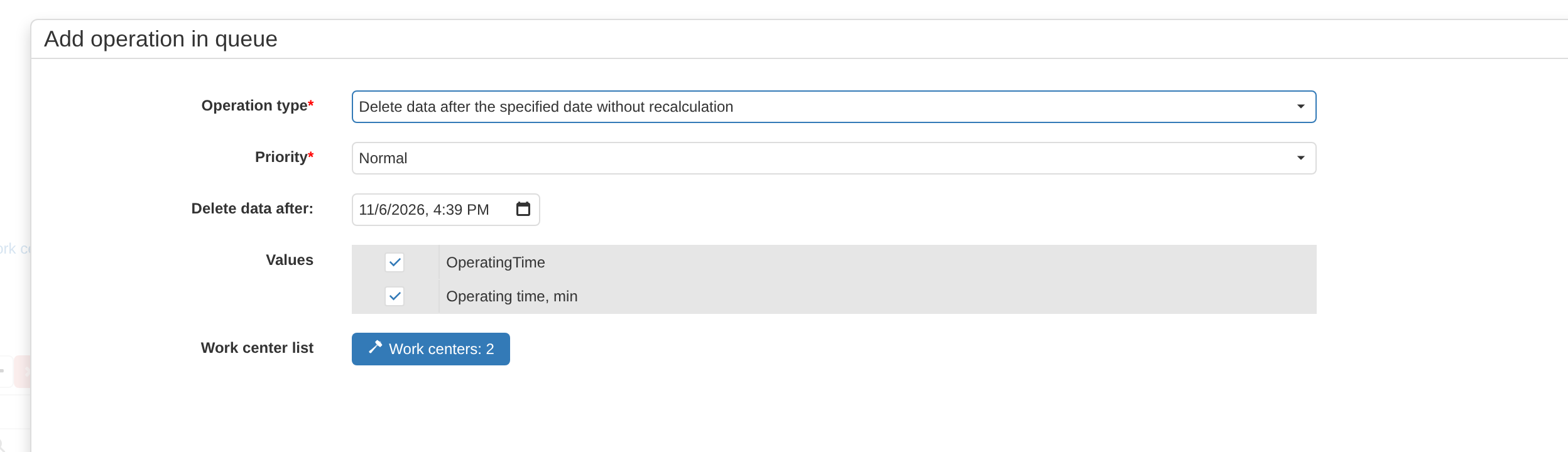
Recalculation from a date starts with an explicit choice of the time boundary, values and Work centers. The operation deletes exactly the selected series; dependent Derived values must be added to the selection separately.
The phrase “without recalculation” applies directly to the deletion operation: it removes stored intervals rather than synchronously calculating new ones in the same dialog. When the operation finishes, an active KPI context resumes. For series whose stored boundary was moved backward, KPI can retrieve source history again or reproduce dependent calculations from the specified date.
Selecting values for such a recalculation requires taking formula dependencies into account. The operation deletes exactly the selected series and does not automatically add dependent Derived values.
For example, suppose two series are stored:
| |
If the Echo formula is changed to Run + 100 and then only the Run history from some date onward is deleted, stored Echo history from that date onward remains unchanged. The new Run history is rebuilt, but the already existing Echo series is not automatically recalculated over its own later stored boundary.
Therefore, when correcting a historical source series, delete from the same date:
- the Basic value or intermediate Derived value being changed;
- every stored Derived value that depends on it directly or through other formulas;
- for a long or unclear dependency chain, use a full clear and recalculation instead of selective recalculation.
If the source series are correct and only the formula of one stored Derived value has changed, you can move that value and every stored value depending on it backward. KPI reads the stored input series and rebuilds the deleted portion of history using the current formulas.
Full recalculation
Use Delete all data and recalculate from scratch when all stored history must be built using the current configuration. This is the most unambiguous option after a change in fundamental formula logic, a large-scale source change, or whenever the complete set of dependent series for selective recalculation is difficult to determine.
After a full clear, calculation begins from the current KPI context Start date. Before starting, check that date and verify that the source history is available in DPA Host. The longer the period and the more Work centers and values involved, the more data KPI must retrieve and recalculate.
A full recalculation is especially important after changing a formula when old and new values must not coexist in the same history. A restart alone applies the new formula only to future calculation; a full clear forces stored history to be rebuilt using one current configuration.
Deleting an old portion of history
Delete data before the specified date without recalculation is intended for the opposite task: discard the early part of history without moving the current calculation boundary backward. Select the date, values and Work centers whose history should be shortened.
After this deletion, an ordinary restart does not restore the deleted older portion merely because it lies after Start date: the series retains a later stored boundary. Use this operation when early history is genuinely no longer needed, not as a way to correct past data.
What to choose in typical situations
| Task | Action |
|---|---|
| Apply a changed formula or source only to future calculation | Restart the KPI context. |
Recalculate one changed stored Derived value from time T | Delete its history from T onward and the same portion of history for every stored value that depends on it. |
Correct source data from time T | Delete from T onward the changed input and every dependent stored series. |
| Repair an internal gap in history | Move the boundary of the affected stored series back to the beginning of the gap; an ordinary restart alone is insufficient. |
| Bring all history in line with the current configuration | Delete all data and recalculate from scratch. |
Intentionally discard old history before T | Delete data before the specified date without recalculation. |
Safe recalculation is therefore determined not only by the date but also by the dependency chain. Every stored time series has its own historical boundary. A restart rereads the configuration, while storage operations determine which portion of history KPI should treat as already existing and which portion it can build again.
8. Analytics “26. KPI”
Analytics → 26. KPI shows final Derived value results for a selected period. KPI does not build a new history stream here: analytics takes the already stored time series, evaluates the required avg, sum, dur and other parts of formulas for the selected period, and shows the overall result together with results for individual Work centers.
Only Derived values with Is general enabled appear in this analytics view. Basic values are not displayed here directly. If an Is general Derived value remains a time series and does not itself contain avg, sum or dur, KPI automatically takes its time-weighted average over the selected period when a final value is requested. Therefore, when a result needs a different aggregate meaning, specify the aggregation explicitly in the formula.
Selecting data for analytics
At the top of the page select:
- KPI context — determines the available values and equipment;
- Work centers — determine the equipment included in the overall request and in the per-equipment comparison;
- a period — for example Day, a shift, or a custom range;
- the date or range boundaries;
- when necessary, particular shifts within the selected calendar period.
The refresh button requests the results again for the current filters. Changing the period or the equipment set does not start a historical recalculation: it only changes the interval over which analytics reads already available KPI data and evaluates the final formulas.
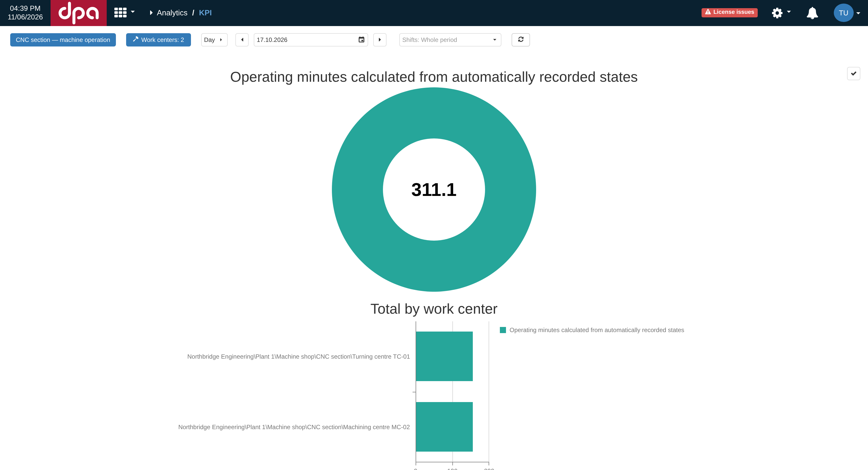
Analytics → 26. KPI: select the KPI context, Work centers, and period at the top. The upper chart shows the overall result for the selected set, while Work center totals shows the same KPIs separately for each selected Work center.
The example shows the general value Work, min = sum(Work) * 60. The upper result 1275.7 applies to both selected Work centers over the selected period. The lower Work center totals chart shows the result separately for each center. For this formula, the overall result really does add the equipment work durations. For an average or a more complex formula, the overall result is determined by the formula itself over the selected set of time intervals and must not automatically be interpreted as a simple sum or arithmetic mean of the lower bars.
What determines how a result is displayed
The Derived value fields described in section 5, “Formulas” are used here as presentation metadata:
| Setting | How it appears in Analytics → 26. KPI |
|---|---|
| Is general | Includes the value in this analytics view. |
| Display name | Used as the result title instead of the technical variable name. |
| Value format | Determines how the number is shown: ordinary number, percentage, or duration. |
| Color | Used in the chart and legend. |
| Sort index | Determines the relative order of general values. |
| Values group | Combines several general values into one upper chart. |
| Equipment values group | Controls grouping of the lower charts by Work center; <Don’t show> excludes the value only from the lower comparison. |
If Values group is not set, a general value gets its own upper chart. For a value expressed as a fraction, you can select percentage formatting: 0.82 is then displayed as 82%. For non-normalized quantities — for example minutes, item counts, or another arbitrary result — rely primarily on the number in the center and the selected value format rather than treating the ring as a mandatory 0-to-100% scale.
If several general values are assigned to the same Values group, they become sectors of one chart. Each sector uses its own Color, the group name becomes the chart title, and the number in the center is the sum of the displayed values. This mode is convenient, for example, for complementary state shares that should add up to 100% when the period is covered correctly.
The lower part of the page shows the same results for individual selected Work centers. If Equipment values group is not set, values are shown in the standard Work center totals chart. The same non-empty group name collects the corresponding series into a separate lower chart with that title. <Don’t show> excludes the value from the lower comparison while preserving its overall upper result.
Data slices
A Data slice lets the same general KPI be calculated separately by time-dependent categories, for example shifts, operators, products, control programs, or downtime reasons. A Data slice is itself a time series: during calculation, KPI intersects its intervals with the intervals of the measured value, so the category is determined for the corresponding part of time rather than attached to the result afterward as a reference attribute.
If Data slices are configured in the KPI context, an additional slice selector appears above the results. One slice can be marked as the default; No slice is also available. After a slice is selected, analytics splits general values that are not combined into a Values group by the values of the selected slice and uses the names and colors of its categories in the charts.
For example, with a shift slice the formula avg(IsProduction) remains unchanged, but the result can be viewed separately for each shift over those portions of time where the corresponding shift was active. If several KPIs have already been combined into their own Values group, the sectors of that upper chart represent the values in the group themselves and the result is not split into additional sectors by the selected slice.
Time coverage and the overall result
Final analytics preserves the time semantics of formulas. A value of 0 participates in the calculation as a number, while a portion with no stored interval does not become zero. Incomplete coverage can therefore change not only an individual Work center result but also the overall result for the selected equipment set.
For avg, the average is weighted by the duration of the existing coverage; sum integrates the area of existing intervals; dur returns their total duration. When several Work centers are selected, the overall result is calculated over their selected periods as one formula request. Before comparing totals, therefore, check that the participating series have comparable and expected time coverage. A control value based on dur is especially useful when a missing portion of history could otherwise look like a plausible number.
Calculation state and errors
A request-state indicator is shown on the right side of analytics. After a successful calculation it returns to its normal state.
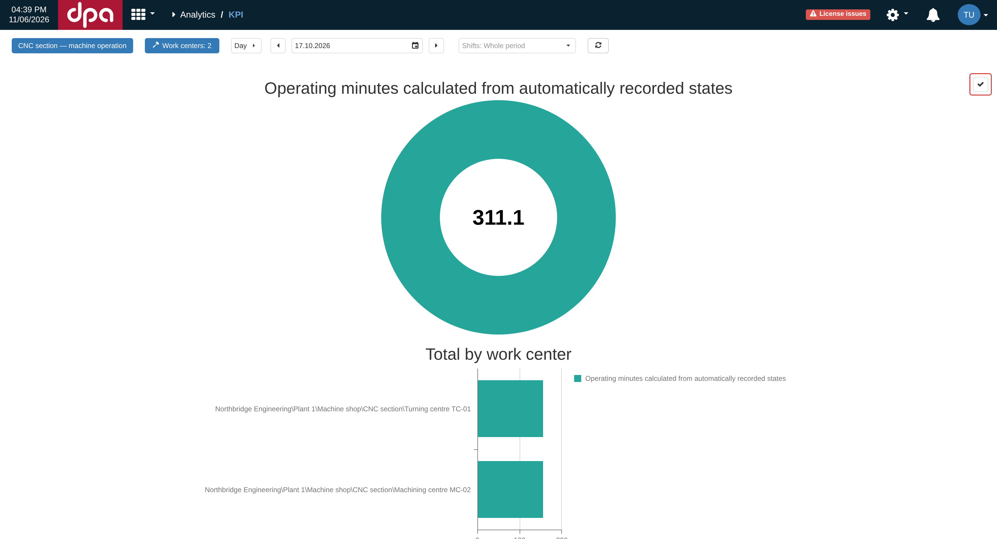
The request-state indicator is located on the right side of analytics. In its normal state it shows a check mark; when an error occurs, the same control opens diagnostic information.
If one of the formulas cannot be evaluated, the corresponding KPI result can be shown as No data, and the error indicator opens diagnostics containing aggregation requests and formula messages. An error in one value does not necessarily mean that every other result on the page is unavailable.
The detailed troubleshooting sequence — from source history and formulas to coverage and service state — is given in section 10, “Troubleshooting an incorrect or missing result”.
9. Analytics “26.1. KPI-timeline”
Analytics → 26.1. KPI-timeline shows stored KPI history on a common time axis instead of one final result for a period. This is the main difference from Analytics → 26. KPI: there formulas are reduced to final numbers for the selected period, while here you can see exactly when a time-series value changed and how a calculated series relates to its source data.
At the top of the page select a KPI context, one Work center, and a period. The timeline is built for one Work center: several pieces of equipment are not combined into a single graph here. The refresh button rereads stored intervals for the current settings; it does not start a historical recalculation.
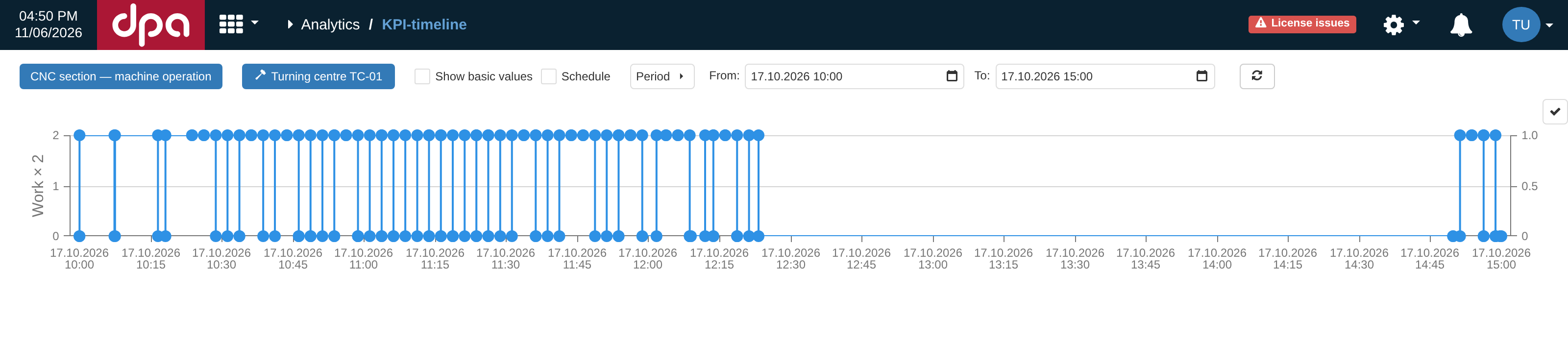
Analytics → 26.1. KPI-timeline: for the selected KPI context, one Work center, and period, every available Derived value gets its own panel. In the example, the stored time series Work × 2 is shown without Basic values.
Which values appear on the timeline
The page creates a separate panel for every Derived value in the selected KPI context. The Is general checkbox, which determines participation in Analytics → 26. KPI, is not a filter here: the timeline considers all Derived values in the context. The variable name is used as the panel title, and the line color comes from the Color field.
A panel does not necessarily contain a line. Analytics → 26.1. KPI-timeline reads stored time-series intervals. An ordinary time-series formula such as B = A * 2 can therefore have its own history and appear on the graph. A formula containing avg, sum, or dur reduces history to a result for the requested period and does not create its own time series: such a Derived value can have an empty panel in Analytics → 26.1. KPI-timeline while still calculating normally in Analytics → 26. KPI.
For the same reason, Store values in storage matters. If actual values of a time-based Derived value are not stored, the timeline cannot reconstruct its past line from the formula text alone. Store a series when you need to inspect its history later or aggregate it over arbitrary periods.
Comparing the result with source series
Show basic values adds the Basic values of the selected KPI context to the timeline. This is useful when checking a formula: you can see the input and the calculated series at the same time, compare switching moments, and find the point from which the result stopped following the expected relationship.
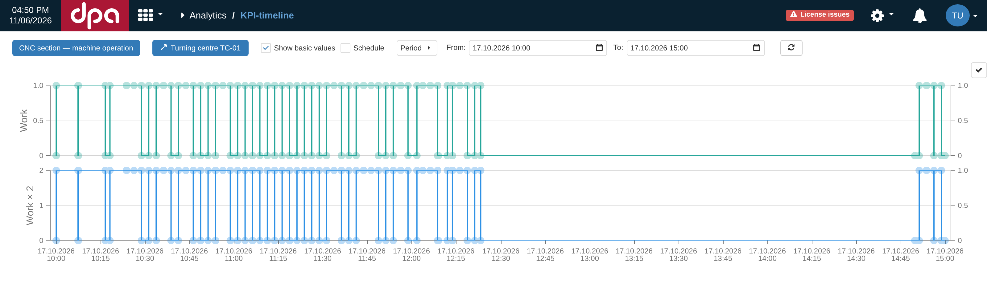
Show basic values adds the source Basic values to the Derived values. Here the upper Work series and lower Work × 2 series have the same interval boundaries, making it easy to see how the formula result follows the source history.
In the example Work × 2 = Work * 2, both panels change at the same time boundaries while the numeric scale of the calculated series is doubled. For a formula that uses several time series, the same view helps show where each input changed and over which common portion the resulting line could change.
The checkbox adds Basic value descriptions to the page, but a useful line still requires stored history. If the source series was not stored or there is no data in the selected period, its panel can remain empty.
Intervals, gaps, and values at a point in time
The timeline displays interval history. A horizontal segment means that the value was active over the corresponding time interval; a transition appears at an interval boundary. The crosshair and tooltip help read the value at a particular moment.
A missing interval is not interpreted as 0. Intervals whose value is NaN are not drawn, and a real gap between adjacent portions breaks the line: the UI does not connect data across a missing fragment. An empty area on the graph should therefore be checked as possible missing coverage rather than treated as a zero value.
If Schedule is enabled, colored shift intervals from the selected Work center schedule are added over every panel. This lets you compare KPI changes with shifts and working-time boundaries without changing the stored values themselves.
Large periods and empty panels
The page loads a limited number of intervals for one series — 50,000 by default. If the selected period contains more history, the state indicator on the right changes to a warning state and reports which series were shown incompletely. In this case, reduce the period or, when high detail is not continually required, use a prepared downsampled time series as described in section 5, “Formulas”.
An empty panel does not always mean a formula error: an aggregating value also has no time history of its own. If a calculation really did fail, the right-hand indicator changes to an error state; its dialog shows the problematic Derived value and the formula message. Distinguishing an error from missing stored history is useful before moving on to deeper diagnostics.
The detailed sequence for checking formulas, source series, coverage, and the state of a KPI context is given in section 10, “Troubleshooting an incorrect or missing result”.
10. Troubleshooting an incorrect or missing result
It is easier to troubleshoot an incorrect KPI by following the data chain rather than starting from the assumption that “the calculation is broken”. The same visible symptom can originate at different levels: source history may be missing, a formula may not produce a time series, stored history may be stale after a formula change, the period may be only partly covered, or final analytics may aggregate the data differently from what was expected.
A useful localization rule is:
- if the Basic value is already incorrect, start with its source and time history;
- if the Basic value is correct but a time-based Derived value is not, check the formula, storage, and the running calculation;
- if both time series are correct but the result in
Analytics → 26. KPIis unexpected, check aggregation, period coverage, the selected Work centers, and the Data slice.
First capture one reproducible example
Before changing settings, record one concrete example: KPI context, Work center or set of Work centers, period, value name, expected result, and actual result. Also note where the problem appears — in Analytics → 26. KPI, Analytics → 26.1. KPI-timeline, a report, or several places at once — and what changes were made shortly before it appeared.
This prevents different causes from being mixed together. For example, an empty panel for an aggregating value in Analytics → 26.1. KPI-timeline may be normal, whereas No data for the same value in Analytics → 26. KPI already requires checking the formula or input history.
| Observation | First check |
|---|---|
| Neither the Basic value time series nor the Derived value series exists | The Basic value source, its mapping to the Work center, the selected period, Data delay, and whether history actually arrives |
| The Basic value exists but the Derived value series does not | Formula, Store values in storage, diagnostic indicator, and whether the context was restarted after the formula changed |
| Time series look correct but the final result is No data | Formula type, arguments of avg / sum / dur, the diagnostic message, and whether stored history exists for the aggregated series |
| A final result exists but looks wrong | Time coverage, selected Work centers, Data slice, units and meaning of the formula; then compare the overall result with individual Work centers |
| An old period remains wrong after a formula is corrected | Historical recalculation is required: an ordinary restart does not rewrite previously stored history |
| The KPI context is enabled but new values do not appear | Check whether input and calculated series actually advance; Enabled by itself does not confirm that every formula and source is operating correctly |
1. Check source history
Open Analytics → 26.1. KPI-timeline for one problematic Work center and enable Show basic values. First find the inputs on the time axis on which the formula depends.
If the required Basic value is absent or its history ends earlier than expected, changing the formula is premature. Check the selected source, its additional parameters, and its mapping to the Work center. For an Indicator source, remember in particular that one variable can be mapped to different Indicators on different Work centers.
Take Polling interval and Data delay into account. The latter deliberately prevents calculation from using data that is too recent, so the expected edge of history can be earlier than the current time. A real gap inside an already processed period is different: it does not automatically become zero.
2. Compare the input and the calculated time series
If input history is correct, find the corresponding time-based Derived value. For a simple relationship such as B = A * 2, interval boundaries of A and B should coincide and the values should follow the formula. With several inputs, the result can change at a boundary of any participating series.
If a panel exists but has no line, check the type of formula. An expression containing avg, sum, or dur is a final calculation for a period and does not create its own time history. For an ordinary time-series formula, check Store values in storage: without stored history, the past line cannot be reconstructed in analytics from the formula text alone.
3. Use formula diagnostics
When calculation fails, the state indicator on the right changes to an error state. Open it: interactive analytics shows the problematic Derived value and a message related to evaluating its formula.
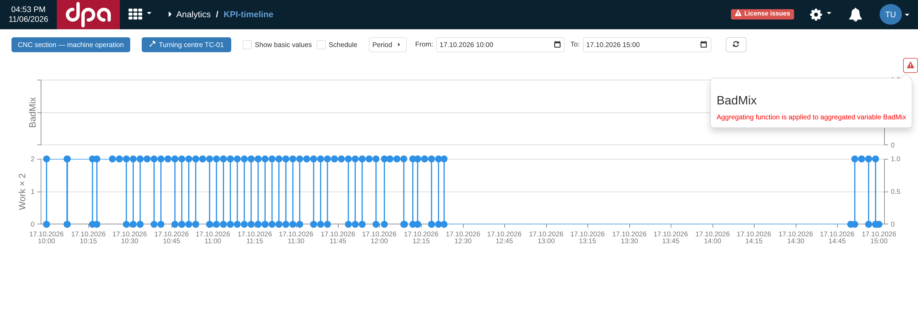
The red state indicator opens formula diagnostics. In the example, BadMix cannot be evaluated and the dialog directly reports incompatible use of an aggregating result; other panels on the page can continue to display independently.
Compare the message with the rules in section 5, “Formulas”. Common causes include an unknown variable name, mixing a final aggregated value with a time series, or passing an invalid argument to avg, sum, or dur. Saving a value card does not by itself guarantee that every entered formula can be evaluated by the running calculation.
If the formula was changed in an enabled KPI context, make sure that the new configuration has actually taken effect in the running calculation. For changes that require a restart, the saved card and the running calculation can temporarily refer to different revisions of the formula.
4. Check time coverage before comparing numbers
For avg, sum, and dur, not only the numerical value matters but also the portion of time for which history actually exists. 0 is a value that participates in calculation; a missing interval is missing coverage. Two results that look similar can therefore have been calculated over different amounts of history.
If a value is expected to cover the entire period, it is useful to create a temporary control Derived value using dur(SeriesName) and compare its coverage duration with what you expect. This is especially useful with several Work centers or a group of mutually exclusive states.
Do not infer coverage only from a visible 0 in a final chart: some views can show an absent value as a zero contribution. It is more reliable to inspect time history in Analytics → 26.1. KPI-timeline or calculate a separate duration with dur.
With several Work centers, the upper result in Analytics → 26. KPI does not have to be the simple arithmetic mean of the values displayed below. The formula is evaluated over the selected periods and equipment as one final request; when coverage differs, individual Work centers can have different effective weights. A strange overall result with plausible individual bars is therefore a reason to compare coverage before investigating rounding.
The same rule applies to Data slices: a category applies only to intervals where the slice itself has history. If a result changes after a slice is selected, check the slice’s time coverage and categories over the problematic period.
5. Distinguish restart from correcting history
Restarting a KPI context rebuilds the running calculation using the current configuration but does not rewrite history that has already been stored. After a formula is corrected, new values can therefore be calculated correctly while an older period still contains results produced by the previous formula.
When history must be corrected, use the operations described in section 7, “Calculation and recalculation”. When recalculating from a selected date, include not only the changed input series but every stored Derived value whose history depends on it. Selectively deleting only the source series does not automatically delete already stored history of dependent values.
If the dependency chain is long or it is not clear which stored series are affected, a full recalculation from Start date is safer than leaving a mixture of old and new calculation revisions.
6. Do not treat the Enabled state as proof that calculation is correct
An enabled KPI context means that its configuration is intended to run. It does not automatically prove that all formulas were built successfully for every Work center, that every source continues to supply data, or that all time series keep advancing.
If the UI shows an enabled KPI context but history is not accumulating, check the actual last boundary of Basic values and Derived values in Analytics → 26.1. KPI-timeline, the diagnostic indicator, and recent configuration changes. If all inputs have stopped together, investigate the source or the connection to DPA Host. If inputs continue but one calculated series stops, return to its formula and dependencies.
Short diagnostic route
For most support cases, the following sequence is enough:
- record one Work center, period, and value for which the problem is reproducible;
- in
Analytics → 26.1. KPI-timeline, check the source Basic values; - in the same view, check the stored time-based Derived value;
- open the diagnostic indicator and rule out a formula error;
- check time coverage and, when necessary,
dur; - only then investigate the final result in
Analytics → 26. KPI, grouping, and Data slices; - if the configuration changed recently, determine whether a restart is sufficient or a historical recalculation is required;
- if the data still does not advance, give the administrator the exact KPI context, Work center, period, formula, observed last history boundary, and diagnostic message.
This order preserves the important distinction between three questions: what arrived at the input, what the running calculation stored, and how analytics reduced stored history to a final result. Checking these levels separately usually makes it possible to find the cause without randomly trying settings.